Simulation #3: Bending of 2D beam under static force (part 1 - theory of mechanics for beam)

I. Introduction

Previous simulation #2 was related to phenomenon of ball in gravitational field about which we were teached at school. Formulas describing the ball movement are known and simple (they do not contain derivative equations in their basic form). Any quantity like x(t), y(t), V(t) etc. can be expressed by its own formula, which mathematicaly is same simple.

This blog is about numerical methods. Numerical methods are used to solve formulas that does not have analytic solution or they are very difficult to find. For instance formulas describing physical phenomenon occurring on the top of a body with irregular geometry. If it is possible to find analytically, it would take much time.

This article is related to simulation from area of structural engineering. We will consider the case of 2 dimentional beam under static force. Formulas describing it are complex and analytical solution may be difficult to find. Luckily, numerical methods are our helpful friend. We will use Finite Element Method (FEM) to find approximate solution - values of different parameters that describe the beam.

II. 2D beam - theory

This article is theoretical and provide required understanding about theory of the beam, from the field of mechanical engineering. The next part will be introduction to FEM method. Theory will be limited to particular case that we deal with as topic is too large to provide lecture for any beam case in one article.

1. What is beam?

First question you may ask is: what is beam? According to Wikipedia:

a beam is a structural element that primarily resists loads applied laterally to the beam's axis (an element designed to carry primarily axial load would be a strut or column).

What is specific for beam and different from other structural elements is that it has one dimention much longer than than other two. For 2 dimentional case, its lenght is much longer than its high. Below picture presents beam that will be modeled. That case has its own name - cantilever beam. It is a beam fixed on one left edge (for example bolted to the wall) and the right edge is free. Static force is acting on the right edge downwards.

Fig 1.1 2D beam with length L and applied force $\vec{P}$. What is typical for beam - external force is applied perpendicularly to beam axis $x$. Beam here is in the state before simulation (before it is bent).

Fig 1.1 presents the initial state (before simulation). After simulation beam bends under acting force $\vec{P}$ or in language of engineering - displacement occurs. Fig. 1.2 presents that state of simulation:

Fig 1.2 2D beam from fig. 1.1, state after simulation.

2. Static equilibrium

To start beam analysis we need to introduce fundamental term of static equilibrium. Statics (or Engineering Statics) is part of Engineering Mechanics that deals with rigid bodies (such as beams) that are in equilibrium state. Equilibrium means that they are not moving. According to Newton's Law, body is not moving when:

• there are no forces acting on body,
• all forces acting on the body are balanced.

We know that first case is not what relevant to our beam as there is force $\vec{P}$ acting on it. Regarding second bullet, it is met when:

1. sum of projections of forces onto x-axis is zero: $$\sum F_x=0\qquad\qquad (1)$$
2. sum of projections of forces onto y-axis is zero: $$\sum F_y=0\qquad\qquad (2)$$
3. sum of moments at any point is zero: $$\sum M_i=0\qquad\qquad (3)$$

Above equations are called external equilibrium equations (for 2D structure). Our 2D beam case, is the system, in which we have 3 degrees of freedom: movement along x-axis, movement along y-axis and rotation. They are related respectively to equations: 1st (moving along x-axis), 2nd (moving along y-axis) and 3rd (rotation).

3. Quantities describing beam

There are multiple quantities describing beam. Three especially important are:

• displacement - (in Polish: przemieszczenie) movement of a point that belongs to a beam due to its bend caused by external force. Below figure presents displacement of point A (point is marked as A' after displacement).

  

  Fig 3.1 Displacement of point A as effect of acting force.

  It can be seen that force $\vec{P}$ causes mainly displacement of y component of the point denotes by v. Displacement of x component denoted by u is relatively much smaller. It makes sense as force $\vec{P}$ acts perpendicular to y axis. We can introduce function v(x) which represents displacement function in y-axis direction (u deflection is much smaller, therefore we can skip it). Below picture presents v(x), we can call it deflection/displacement curve:

  

  Fig 3.2 Deflection function for bending beam.

  Based on above figure true is that: $$v(x)=\frac{d\theta}{dx}$$ At the end of this article we will derive formula for v(x) for our beam.
• stress - (in Polish: naprężenie) denoted as $\vec{p}$ it is vector expressing the intensity of internal force. It can be describe as force per unit area or intensity of forces distributed over given section. Internal forces in the beam are effect of external force (force $\vec{P}$ in our case). Stress vector $\vec{p}$ is sum of two vectors - normal stress vector ($\vec{\sigma}$) and sheer stress vector ($\vec{\tau}$): $$\vec{p}=\vec{\sigma}+\vec{\tau}$$
• strain - (in Polish: odkształcenie) denoted as ($\epsilon$) it is the change of displacement per unit length: $$\epsilon = \frac{\text{final_length} – \text{initial_length}}{\text{initial_length}}$$

Stress expresses the internal forces that neighbouring particles of a continuous material exert on each other, while strain is the measure of the relative deformation of the material. But what is relation between them?

4. Stress strain relation

Beam behaviour under the force to some extent is similar to spring behaviour under the force. Commonly known is law, which says that spring deflection from equilibrium (state without force) is proportional to force applied. It is called Hooke's law. For the beam it is analogical equation, which is applicable for small deflections: $$\sigma = E\cdot \epsilon,\qquad\qquad (4.1)$$ where:

E – is Young modulus, which is measured by experience. It is constant value specific for material that beam is made from.

Below figure presents relation between strain and stress (stress – strain curve):

Fig 4.1 Stress–strain curve for steel (picture from Wikipedia)

We would like to apply enough small force that beam can behave as linear-elastic solid (in range from 0 up to point 2 in above fig.). In that range formula (4.1) is applicable.

5. What forces are acting on the beam?

We mentioned in previous section that there are 2 types of forces - external and internal. Below picture (5.1) presents types of forces that are acting on the beam. In part a) there is external static force $P$ that we already know. Another external force is force $R_A$, which is reaction force caused by fixed support (wall).

Fig 5.1 External and internal forces acting on bending beam.

When we cut beam into two parts at x – we have left and right part that reacts on each other by inner forces in the crosssection. Those forces are equal but acts in opposite direction. Therefore we can consider only left part of the beam – fig 5.1 b). In its crosssection we can define small section called $\Delta h$, then we can say that $\Delta P_w$ is total force that acts on that section as reaction of external forces acting on beam. $\Delta P_w$ is internal force. It is related to stress value. Let's figure out this relation.

When we limit size of $\Delta h$ to zero: $$\lim_{\Delta h \to 0} \frac {\vec{\Delta P_w}}{\Delta h} = \vec{p},$$ where p is called stress vector. It is intensity of internal force at specific point. In 2D case crossection is just line therefore p depends only on y: p(y). Stress vector $\vec{p}$ is sum of two vectors: normal stress vector ($\vec{\sigma}$) and sheer stress vector ($\vec{\tau}$) as we state before. Those 2 types of stress corresponds respectively to 2 types of internal forces: normal force and sheer force.

We can calculate average vector of p for the whole crosssection when we calculate it in its centroid (center of mass/center of an area, in our 2D case it is center of crossection y=0). Total $p$ is marked as $P_w$ and presented at fig. 5.1 c). When we cast it on x and y axis, we get respectively total normal force N and total sheer force T for that crossection. Their values are: $$N=\int \limits_{h} \sigma dy,$$ $$T=\int \limits_{h} \tau dy,$$ where integral is calculated on crossection which in this case is (2D) line segment with lenght h. There is relation between $P_w$ and external forces acting on beam: $$P_w+\sum \limits_{i}P_{li}=0,$$ $$P_w+\sum \limits_{i}P_{ri}=0,$$ where $P_{li}$ are vectors of all external forces acting on left part of the beam, $P_{ri}$ are all external forces vectors acting on right part of the beam. It make sense that, we can calculate internal force $P_w$ considering either left or right part of the beam, because both of them stays in static equilibrium.

Above equation can be rewrite as: $$P_w=-\sum \limits_{i}P_{li},$$ $$P_w=-\sum \limits_{i}P_{ri}.$$

6. What moments are acting on the beam?

Now it is time to consider moment of forces that are acting on our beam. On the left we have wall into which beam is attached. In the language of Statics it is fixed support (cantilever). This kind of support produce both reaction force and reaction moment $M_A$ as well – figure 6.1 a). How to understand reaction moment? Imagine you are holding a long board by one end and lifting the other end. Where you hold it, you have to rotate your wrist to keep the board balanced. The same happens with the moment in a cantilever. Why does this happen? This is due to the balance of forces and moments. Introducing a reaction moment helps the beam maintain balance by counteracting the forces and moments acting on it. Therefore $M_A$ has orientation that makes it counteracting of bending of the beam.

Fig 6.1 Moments acting on bending beam.

Analogically as previously, lets cut the beam into two parts left and right (figure 6.1 b)). We can see, that in its crossection, there is another moment called bending moment Mb. In the right part there is moment with same lenght but acting in oposite direction to balance the one from left part in given crossection. There is relation between $M_b$ and moments of external forces like for example moment with relation to point $M_A$: $$M_b+\sum\limits_{i}M_{li}=0,$$ $$M_b+\sum\limits_{i}M_{ri}=0,$$ where $M_{li}$ are all moments of external forces acting on left part of the beam, $M_{ri}$ are all moments of external forces acting on right part of the beam. Therefore: $$M_b=-\sum\limits_{i}M_{li},$$ $$M_b=-\sum\limits_{i}M_{ri}.$$ Notice that it is sum of vectors.

7. Sign convention.

Below figure describes sign convention that are valid in Statics for quantities like: $M_b$, T, N.

Fig 7.1 Sign convention for normal force, shear force and bending moment.

Sign of moment which is defined with respect to a fixed reference point, for example $M_A$ (with respect to point A) is determined differently than sign of bending moment $M_b$:

Moment M is positive if it is rotating clockwise:	Moment M is negative if it is rotating counterclockwise:
Fig 7.2 a) Sign of moment in relation to point is positive when it is rotating clockwise.	Fig 7.2 b) Sign of moment in relation to point is negative when it is rotating counterclockwise.

8. Finding reaction force $R_A$, reaction moment $M_A$, sheer force $T$ and bending moment $M_b$

If we ignore wall on the left, but take into account moment and reaction that it is causing, we can try to calculate forces $R_A$, $M_A$ using equilibrium equations.

Fig 8.1 Forces, moments and its reactions acting on bending beam.

From equilibrium equations we have:

ad. 1) $\sum F_x=0 \quad \implies 0=0$ (no external forces along x-array)

ad. 2) $\sum F_y=0 \quad \implies -P+R_A=0 \implies R_A=P$

ad. 3) lets consider point x=0; y=0. Moment in it should be zero: $$\sum M_{(0;0)}=0 \quad \implies P \cdot L–M_A=0 \implies M_A=P\cdot L$$ $M_A$ and $R_A$ values we can use now to calculate $M_b(x)$ and $T(x)$. They can be determined when we split beam into 2 parts – left and right and considerint moments and forces only from left part. As mention before, we are allowed to consider left part only due to fact that it is in static equilibrium. It is possible to analyze right part of course and it should give the same results. For the crossection of cut (at x in above fig.), bending moment is equal to sum of all moments from left part of the beam in respect to center point of that crossection ($y=0$): $$M_b(x)=R_A\cdot x-M_A = P\cdot x - P\cdot L= P(x-L)$$ According to sign convetion $R_A$ force makes beam bent upwards so its moment's ($R_A\cdot x$) sign is positive, moment $M_A$ whereas makes beam bent downwards, so its sign is negative.

Sheer force T at x is equal to sum of forces acting along y-axis on the left from crossection: $$T(x) = R_A = P$$ According to sign convention figure, $R_A$ force is positive, because it is on the left from crossection and it is pointing upwards.

$T(x)$ can be confirmed using relation $T(x) = \frac{dM_b(x)}{dx}$ (Schwedler's Theorem). It is equal to P, therefore value is right.

Now we can draw graphs for both cases:

Fig 8.2 Bending moment and sheer force plots for bending beam.

As we were able to calculate reaction forces and moments using equilibrium equations, therefore we can say that beam is statically determined.

9. Beam bending classification

When beam bending happened due to moment only (when sheer force T is zero) we call it pure bending. Then crossection shape remains flat during bending. When sheer force exists also then bending is called non-uniform. Sheer force makes bending more complicated, when it is strong comparing to beam strenght against lateral force and crossection shape may be distorted during bending instead of remaining flat. We can see, that in our case bending moment $M_b$ is non-zero for all beam lenght (except from point $x=L$) and also sheer force T is non-zero. It is very difficult to calculate in such case analitically beam parameters like stresses, displacement function. We are able to do this numerically using finite element method. However for now, let's perform analytical calculations applying common simplification, used when lenght of the beam is much greater than its width, and then impact of sheer force can be skipped. We will use this simplification when calculating formula for normal stress. So we will assume that bending is pure: $M_b\neq 0$, $T=0$.

In such model, we can imagine the beam to be made up of longitudinal fibers parallel to the longitudinal axis of the beam. Each fiber has crossection $\Delta h$ and lenght L. Fibers does not acts on each other along lateral direction (y-axis).

10. Normal stress formula deriviation

Fig 10.1 Beam fragment for normal stress formula deriviation.

In above figure it is presented small part of bending beam. We can see that upper edge of that beam fragment ($y=h/2$) gets expanded, whereas bottom edge ($y=-h/2$) gets compressed. Because one edge extended and opposite one compressed, therefore there should be a fiber between them that does not change its length when beam is bending. With blue line I marked, so called neutral axis, which is that particular fiber. In case of beam with regular rectangular shape (our beam), neutral axis is at the center of crossection ($y=0$). In further part of this article, we will see why it is like that. We assume that face of the cut $|BD|$ remains plane (pure bending), and it remains perpendicular to the deformed axis of the beam (neutral axis).

Above beam fragment we will use to derive formula for bending stress $\sigma$. Firstly, let's write what is the length of upper edge of beam fragment: $$\epsilon = \frac{\text{final_length} – \text{initial_length}}{\text{initial_length}}$$ We assume that blue line (neutral axis) does not change its length so it has initial length after bend. Its length is: $$\text{inital_length} = |EF| = \theta \cdot R$$ $$\text{final_length} = |AB| = \theta \cdot (R+ \frac{h}{2})$$ Generally, final_lenght for any fiber is: $$\text{final_length} = \theta \cdot (R+y),$$ therefore strain formula is equal to: $$\epsilon = \frac{\theta\cdot (R+y)-\theta R}{\theta \cdot R}= \frac{y}{R}$$ Note: often in books, in above formula there is minus on RHS. It depends on how we set XY coordinate system.

We are talking about linear – elastic solid, therefore relation between stress and strain is: $$\sigma = E\cdot \epsilon$$ When we substitute $\epsilon$ to above formula, we get: $$\sigma = E \cdot \frac{y}{R},$$ we can see that the highest value of stress we get at the bottom and at the top of the beam, however sign in both cases are different. For extension we have positive, for compression negative. Above formula for sigma depends on radius R. Let's do more transformations and get rid of it. Below figure presents again our beam part with marked $\sigma$ at the right edge of the beam part.

Fig 10.2 Beam fragment, bent due to external force with marked normal stress values on the right crossection.

Because part of the beam is in static equilibrium, we can use static equilibrium equations: $$\sum F=0,$$ because normal stress $\sigma$ is related to distributed force over the crossection, therefore: $$\int\limits_{-h/2}^{h/2}\sigma dy=0,$$ taking out constants: $$\frac{E}{R}\int\limits_{-h/2}^{h/2}y dy=0.$$ It can be seen, that existence of blue line (neutral axis) which we assume before is now proofed because it is determined by integral from above equation of static equilibrium.

For second equilibrium equation:

$\sum M =0$, therefore $$\int\limits_{-h/2}^{h/2}\sigma y dy =M.$$ When we substitute $\sigma$ value: $$\frac{E}{R}\int\limits_{-h/2}^{h/2}y^2 dy=M.$$ Integral in above equation has special name – it is Moment of Intertia I. Therefore: $$M=\frac{EI}{R}.$$ We derived 3 relations so far: $$\epsilon=\frac{y}{R}; \quad \sigma=\frac{Ey}{R}; \quad M=\frac{EI}{R}.$$ We can combine 2nd and 3rd relation to get rid of R parameter: $$\sigma=\frac{My}{I},$$ the above is formula is important relation in Statics and it is called flexure formula. It says, when we know the moment that is applied to the beam and its moment of inertia for particular crossection, then we can calculate maximum stress in it.

For 2D case, moment of inertia I we can called $I_y$ and calculate as: $$I_y=\int\limits_h y^2 dy=\left[\frac{y^3}{3}\right]^{h/2}_{-h/2}=\frac{h^3}{12}.$$ Now formula for normal stress is: $$\sigma=\frac{12My}{h^3},$$ we can finally substitute known value of M calculated before: $$\sigma=\frac{12(Px-PL)y}{h^3}=\frac{12(x-L)Py}{h^3}.$$

11. Sheer stress formula deriviation

Now we are going to derive formula for shear moment $\tau$. Below picture shows both shear force and bending moment acting on beam cut:

Fig 11.1 Shear force and bending moment acting on the beam cut with corresponting shear and normal stresses.

We have seen that the normal stresses due to bending moment M are linearly distributed over the cross section, with maximum magnitudes of normal stress occuring on the outer fibers of the beam and with zero normal stress at the neutral axis (the neutral axis passing through the centroid of the cross section). In our case, shear force T acts along with the bending moment $M_b$ and a component of shear stress will exist. Shear strains correspond to a change in angle of the stress element. This angle change is somewhat in contradiction with the pure bending assumption of the cross section remaining perpendicular to the deformed beam axis. For our normal stress formula, we will assume that the shear strain effects will be slight and that, even in the presence of shear stress, the distribution of flexural stress on a given cross section is unaffected by the deformation due to shear and flexure formula equation is still valid for computing the normal stresses on the cross section.

Suppose we consider a stress element on the side of a beam with a non-zero shear force resultant on the face of the cut (Fig. 11.2). Our goal here is to determine the transverse shear stress component $\tau_{xy}$ that corresponds to the shear force resultant T. Note, however, that since $\tau_{yx} = \tau_{xy}$ (based on the rule that sheer stress in mutually perpendicular planes are equal*), the transverse shear stress component $\tau_{xy}$ is the same as the longitudinal shear stress component $\tau_{yx}$. Stated in different words, we can determine the transverse shear stress by calculating the longitudinal shear stress.

(*) rule is known in Statics, it is easy to proof – try to calculate moment in any point of the element and equal it to zero (according to equlibrium equation).

Fig 11.2 Beam cut element with marked all types of stresses acting on it.

Consider the aribitrarily-loaded beam shown below:

Fig 11.3 Aribitrarily-loaded beam with selected cut.

As can be seen, we isolate a section of the beam between locations $x$ and $x + \Delta x$. Zoom of this part of beam is presented in below figure:

Fig 11.4 Zoom of selected cut from fig. 11.3 with marked forces, moments and stresses.

The the resultant of shear forces and bending moments acting on the beam section is shown in 11.4 a). The resultant bending moments $M(x)$ and $M(x + \Delta x)$ produce normal stresses of $\sigma(x)$ and $\sigma(x + \Delta x)$ on the left and right faces of the beam section, respectively (fig. 11.4 b)).

Normal stress on beam section value is: $$\sigma(x,y)=\frac{-M(x)y}{I}, \\ \sigma(x+\Delta x, y) = \frac{-M(x+\Delta x)y}{I}.$$ Total sheer force resultants on beam section (marked in figure 11.4 a)) is: $$T(x)=\frac{dM}{dx}.$$ Suppose we further isolate a slice of this beam section, found below a given value of y – it is marked as $A'$ in fig. 11.4 c) also present in figure 11.4 d). Sheer stress $\tau$ is related to sheer force. It is acting on both left and right crosssections of the beam part and as well in longitudinal direction (fig. 11.4 d)).

We can define forces at $x$ and $x + \Delta$, acting on slice A' that are corresponding to normal stress $\sigma$: $$F(x)=\int \sigma(x,y)dh', \\ F(x+\Delta x)=\int \sigma (x+\Delta x,y)dh'.$$ Thre is one more force factor along x-axis which corresponds to longitudinal sheer stress. Longitudinal sheer stress acts on the upper surface of the slice at y. Corresponding force to it is marked as $\Delta H$ in fig. 11.4 d).

Because $A'$ element is in equilibrium state, total force along x-axis should be zero: $$\sum F_x=F(x)-F(x+\Delta x)+\Delta H=0 \implies \Delta H=F(x+\Delta x)-F(x).$$ The shear stress corresponding to this resultant shear force is found from the usual definition of stress in terms of the force resultant as: $$\tau=\lim_{\Delta x \to 0} \frac{\Delta H}{\Delta x} =\lim_{\Delta x \to 0} \frac{F(x+\Delta x)-F(x)}{\Delta x} =\frac{dF}{dx}.$$ We can calculate F(x) using below relation: $$F(x)=\int \sigma (x,y) dh'=\frac{M(x)}{I}\int y dh'=\frac{M(x)}{I}\int \limits_{-h/2}^{-y}ydy=\frac{M(x)}{I}\left[ \frac{y^2}{2} \right]_{-h/2}^{-y}= \\ =\frac{M(x)}{I}\frac{1}{2}\left(\frac{h}{2}-y \right)\left(\frac{h}{2}+y\right).$$ Combining above equations gives: $$\tau=\frac{\left(\frac{h}{2}-y \right)\left(\frac{h}{2}+y\right)}{2I}\frac{dM(x)}{dx}=\frac{\left(\frac{h}{2}-y \right)\left(\frac{h}{2}+y\right)}{2I}T,$$ where we used relation (Schwedler's Theorem) $T = dM(x)/dx$.

Moment of inertia $I = h^3/12$ for our beam, therefore final formula for sheer stress is: $$\tau= \frac{\left(\frac{h}{2}-y \right)\left(\frac{h}{2}+y\right)12}{2h^3}T=\frac{\left(\frac{h^2}{4}-y^2\right)6}{h^3}T.$$

12. Displacement function formula

Now it is time to find value of displacement function v(x). Below function, which can be find in books for Statics, is differential equation that describes relationship between displacement function of beam along y-axis (marked as v(x)) with other parameters that we introduced before: $$EI\frac{d^2 v(x)}{dx^2}=-M_b.$$ Substituting value of $M_b$, we have: $$EI\frac{d^2 v(x)}{dx^2}=PL-Px.$$ To find v(x), we need to integrate equation twice.

1st integration gives: $$EI\frac{dv(x)}{dx}=EI\theta=C+PLx-\frac{1}{2}Px^2. \qquad\qquad (12.1)$$ 2nd integration: $$EIv(x)=D+Cx+\frac{1}{2}PLx^2-\frac{1}{6}Px^3. \qquad\qquad (12.2)$$ From border condition we can calculate constant values C and D:

• (from eq. 12.1) for $x=0$, $\theta=0 \implies C=0$,
• (from eq. 12.2) for $x=0$, $v(0)=0 \implies D=0$.

After substitution of constant values and transformations, this yields to final formula of displacement function: $$v(x)=\frac{6Px^3}{Eh^3}\left(L-\frac{h}{3}\right).$$

13. Example

We will solve our beam case for below values:

L=6m
E=20 000 MPa
h=800mm
P=150 kN

Using SymPy Python's library I programmed equations derived in previous chapters for sheer force, bending moment, deflection function, normal stress and sheer stress. Substituting above values, I created graph for each parameter (using Matplotlib library):

Fig 13.1 Sheer force plot for bending beam

Fig 13.2 Bending moment plot for bending beam

Fig 13.3 Displacement function plot for bending beam

Fig 13.4 Normal stress plot for bending beam

Fig 13.4 Sheer stress plot for bending beam

III. Summary

This article was introduction for Mechanics of the beam. In the next part, I will describe basics for FEM method (linear) based on our beam case - so further, we can proceed with the actual simulation.

Simulation #2: Ball motion in gravitational field (part 2 - program)

Previous simulation #1 was visualisation rather than real simulation, because it does not show for user any calculated physical properties. This simulation is different, because:

• it calculates physical properties that describe physical phenomenon (ball motion in gravitational field) with units;
• it compares results with theory, to assess calculation error.

Numerical simulations are used for solving complex equations like differential equations for which finding analytical solutions is very difficult or the solution even does not exists. Ball motion in gravitational field, on the other hand is described by well known simple physics formulas. Therefore numerical methods has no practical usage in that case, because even simple calculator can do the work. However, I introduce numerical methods for this case for educational purpose. I am going to show that we can calculate different physical properties describing ball's motion without using final formulas.

In details, the purpose of program that realizes this simulation is:

• to make possible for user to enter easily initial values of physical properties that describe ball in $t=0$ moment (initial velocity $\vec{V}_0=[V_{x0}, V_{y0}]$ of ball and its initial height $h_0$);
• to make possible for user to enter size of time step $dt$ used in simulation;
• to calculate physical properties that describe ball motion with units (max height $h_{max}$, final velocity $V_{end}$, max distance $d$, time of flight $t_{end}$, time to reach max height $t_{max}$);
• to visualize ball motion (without alignment of time in simulation with clock time, but with alignment with calculation progress);
• to calculate delta between simulated results and theoretical results (based on formulas from part 1);
• to make possible for user to store results from at least one simulation run to be able to compare them with results from other run.

Program/simulation presentation

Below picture (Fig 1) presents UI of the program. It contains 3 radio boxes to select 1 from 3 motions. Each one has related set of input fields in which we can set entry conditions.

Fig 1.

When simulation is finished, results values that describe ball motion are calculated (which is indicated by red outline around resize button). Results can be saved in the second table. It is very useful if we want to compare results between two different simulations. Fig. 2 shows presentation of calculated results:

Fig 2.

Below picture (Fig 3) shows how time step $dt$ size increases/decrease error of calculations. When the time step decreases, the accuracy of calculations increases and vice versa. Using second table we can compare results easily.

Fig 3.

It can be seen that ball does not hit the ground on above pictures. It is because, simulation calculates and visualizes the last step when the ball height is still above the ground: $y\geq 0$. Case $y=0$ for last step happens only for enough small time step value $dt$ or accidentally for larger $dt$ (in lucky cases). The smaller $dt$ is - the closer ball to the ground will be. $dt$ with order of magnitude $10^{-4}$ is enough to reach $y=0$ for all types of motions (all entry conditions). Below picture (Fig 4.) shows results of calculation with $dt=0.0001$:

Fig 4.

It can be seen that calculations are very accurate. Difference between theoretical and simulated values are exactly the same with the 2nd decimal place. Excellent view!

The following figure (Figure 5) shows the possibility of adjusting the angle and distance of the camera setting from the object on the scene in VPython. Change can be done by hold and drag right or both buttons of the mouse:

Fig 5.

It looks interesting and can be useful for example for more visually complex simulations (with many moving objects) like for example model of solar system.

Implementation

To write this program, I used combination of wxPython and VPython libraries. wxPython is library for making UI in Python and VPython is scientific library (for Physics mainly) that display 3D objects and animations. Objects in that meaning are for example: vectors, spheres, cubes.. They can look like 2D, if we do not move them along z-axis, however in fact they are always 3D (it can be seen on Fig. 5). I do not use tkinter library for UI like in Simulation#1, because VPython uses wxPython. VPython usually opens animation in new window and I want to present everything in only one window, so to be able to do this we need to use wxPython.

I) Program structure:

Program consists of two classes: Ball and Simulation. Beyond that, it contains couple of functions whose are related to UI. The following tables contains list of variable and methods with short description about each one:

Class: Ball
Variables	Description
t	time
dt	time step
g	gravitational acceleration
x0,y0	initial coordinates of the ball (for t=0)
vx0,vy0	initial velocity of the ball (for t=0)
x,y	current ball coordinates
vx,vy	current ball velocity
nextY	auxiliary variable, it stores value of y for next calculation's interation
mysphere	Vpython object (sphere) which represents the ball
velocityVector	Vpython object (arrow) which represents velocity vector of the ball
Methods	Description
nextStep	calculates next ball position and velocity after time t=dt

Class: Simulation
Variables	Description
g	gravitational acceleration
ifSimulationWorks	auxiliary variable of boolean type, is True if simulation is already working
simulationCalculatedParameters	dictionary, where keys are physical properties that describe ball motion (hmax, Vend, d, hmin, tend, vxend, vyend) and values are their results
initialData	dictionary, stores: initial position, initial velocity and time step values
Methods	Description
runSimulation	runs simulation
stopSimulation	stops simulation
initEntryData	auxiliary method, reads data from all input fields and store them in initialData dictionary
calculateEndParameters	method calculates physical properties that describe ball motion: hmax, Vend, d, hmin, tmax, tend, vxend, vyend
getTheoreticalResults	method calculates theoretical values for physical properties that describe ball motion: hmax, Vend, d, tmax, tend

Table related to class Simulation does not contain all variables and methods used in implementation. Some of them are UI related and I skipped them.

You can find project files on github: https://github.com/sim-num/BallInGravityField.


II) Steps to program simulation:

1. Set initial ball's position and velocity
2. Calculate position and velocity for next simulation step
3. If calculated position is above the ground accept results, if not - stop simulation
4. Update calculated ball's physical properties
5. Go to step 2

III) Implementation of the steps:

• Ad 1. (Set initial ball's position and velocity)
  
  Initial position and velocity is set by user in proper fields in UI. Then, those values are read by method initEntryData from class Simulation and stored in dictionary initialData:

  
      def initEntryData(self):
          if radio1.GetValue():  #if radio button nr 1 is selected (is true)
              self.initialData={'x0':0,'y0':int(inputH0_1.GetValue()), 'vx0':int(inputVx0_1.GetValue()), 'vy0':int(inputVy0_1.GetValue()), 'dt':float(inputDt.GetValue())}
          if radio2.GetValue():
              self.initialData={'x0':0,'y0':int(inputH0_2.GetValue()), 'vx0':int(inputVx0_2.GetValue()), 'vy0':int(inputVy0_2.GetValue()), 'dt':float(inputDt.GetValue())}
          if radio3.GetValue():
              self.initialData={'x0':0,'y0':int(inputH0_3.GetValue()), 'vx0':int(inputVx0_3.GetValue()), 'vy0':int(inputVy0_3.GetValue()), 'dt':float(inputDt.GetValue())}
  

initEntryData method is called at the beginning of simulation inside runSimulation method from class Simulation (see code in Ad 4.). Then initialData dict is passed to contructor of class Ball to initialize new Ball instance:

class Ball(object):
    ...
    def __init__(self, initialData, dtt):
        self.vx0 = initialData['vx0']
        self.vy0 = initialData['vy0']
        self.x0 = initialData['x0']
        self.y0 = initialData['y0']

NOTICE: "$\ldots$" in code represents some skipped part of the code irrelevant in described context.


• Ad 2. (Calculate position and velocity for next simulation step)
  
  This step is implemented by method nextStep from class Ball:

  
      def nextStep(self):
          self.nextY = self.y + self.vy * self.dt
          if self.nextY > 0:
           self.t+=self.dt
           self.vy = self.vy-self.g*self.dt
           self.x = self.x + self.vx * self.dt
           self.y =self.y + self.vy * self.dt
           ...
  
  

  $V_x$ component of ball's velocity vector is constant, therefore it is not calculated during simulation. What we need to calculate are components of position vector: $x$, $y$ and velocity component $V_y$. They can be denoted by $x(t)$, $y(t)$, $V_y(t)$, because they are time dependent. All of them are calculated numerically for each time step. It is done using above algorithm. This part of algorithm is so important that requires another part of this topic for exmplanation.
  
• Ad 3. (If calculated position is above the ground accept results, if not - stop simulation)
  
  In method nextStep, we check if after calculation of next step, ball position is still above the ground. If yes - then method returns True, of not - then returns False, which is the indicator to stop the simulation.

    def nextStep(self):
        self.nextY = self.y + self.vy * self.dt
        if self.nextY > 0:
         self.t+=self.dt
         self.vy = self.vy-self.g * self.dt
         self.x = self.x + self.vx * self.dt
         self.y = self.y + self.vy * self.dt
         ...
         return True
        else:
         return False

• Ad 4. (Update calculated ball's physical properties)
  
  nextStep method is called inside method runSimulation from class Simulation. After each simulation step, for which ball is still above the ground, as I mentioned previously - nextStep method returns value True. Next, this value is assigned to variable status. Its value is condition for while loop in which we invoke nextStep method and calculateEndParameters method. This last method is responsible for calculation of physical properties that are stored in simulationCalculatedParameters dictionary. The code below shows hierarchy of methods and while loop:

  
      def runSimulation(self, event=None):
          ...
          self.simulationCalculatedParameters={'hmax':-1,'vxend':-1,'vyend':-1,'Vend':-1,'d':-1,'tend':-1,'hmin':1000000}
          ...
          self.initEntryData()
          self.ourBall=gravityFieldBall.Ball(self.initialData, float(inputDt.GetValue()))
  
  
          if self.ifSimulationWorks == False:
              self.ifSimulationWorks = True
              status=True
              ...
              i=0
              ...
              while self.ifSimulationWorks and status:
                  self.calculateEndParameters()
                  ...
                  status=self.ourBall.nextStep()
                  ...
                  i += 1
          ...
          self.ifSimulationWorks=False
          return
  
  

  Code of calculateEndParameters method is presented below:

  
      def calculateEndParameters(self):
          if self.ourBall.y>self.simulationCalculatedParameters['hmax']:
              self.simulationCalculatedParameters['hmax']=self.ourBall.y
              self.simulationCalculatedParameters['tmax']=self.ourBall.t
  
          if self.ourBall.y>0 and self.ourBall.y<self.simulationCalculatedParameters['hmin'] and self.ourBall.vy<0:
              self.simulationCalculatedParameters['hmin']=self.ourBall.y
              self.simulationCalculatedParameters['d']=self.ourBall.x
              self.simulationCalculatedParameters['vxend']=self.ourBall.vx
              self.simulationCalculatedParameters['vyend']=self.ourBall.vy
              self.simulationCalculatedParameters['Vend']=math.sqrt(self.ourBall.vx**2+self.ourBall.vy**2)
              self.simulationCalculatedParameters['tend']=self.ourBall.t
  

  First if condition checks if current y is the largest value found, if yes - then it is stored in simulationCalculatedParameters dict as hmax value with corresponding tmax value to it. The second if condition checks if ball is still above the ground, if current y position component is at the same time the smallest value found . The last part of 2nd condition checks if ball is falling down (Vy velocity component is negative). We need to consider only falling part of the ball motion for searching physical properties like: $V_{end}$, $t_{end}$, $d$. hmin is auxiliary variable, used to figure out if current y position is the lowest position of the ball above the ground (during falling down part).
• Ad 5. (Go to step 2)
  
  This step is realized by while loop inside runSimulation method.

IV) Simulation visualisation

This time I used VPython library for making simulation's visualisation. Because I used it for the first time here, I will list every object I used with quick description:

• display - to combine VPython window with wxPython window, we define display object. It creates VPython scene. To create it, we put window type object from wxPython libary as constructor parameter:

  
  w = window(width=L, height=W,
             menus=False, title='Ball motion in gravity field - 2D simulation',
             style=wx.SYSTEM_MENU | wx.CAPTION | wx.CLOSE_BOX)
  
  #create scene in VPython inside window:
  scene = display(window=w, x=10, y=105, width=600, height=500, center=(40,28,0), background=(0,0,0), autoscale=True)
  

• label - object is used for creating label (for example white box with "h= V=" values):

  
  hV_label = label(pos=(45, 55, 0), text='h=\nV=', xoffset=1, line=0, box=True, opacity=0)
  

  Another example is axis description:

  
  labelX = text(text='x [m]', depth=0.4, color=color.white, height=1.5, pos=[ymax, -3 * tic_h], font='serif')
  

• arrow - object is used for creating axes in XY coordinate system:

  
  xmin = 0.
  xmax = 50.
  ymin = 0.
  ymax = 55.
  
  # tick marks
  tic_dx = 5
  tic_h = 1
  self.xaxis = arrow(pos=(xmin, 0, 0), axis=(xmax+tic_dx, 0, 0), shaftwidth=0.2)        # axes
  
  self.yaxis = arrow(pos=(0, ymin, 0), axis=(0, ymax+tic_dx, 0), shaftwidth=0.2)
  

  The same object can be used to create $\vec{g}$ vector:

  
  self.gravityVector = arrow(pos=(70, 55, 0), axis=(0, -5, 0), shaftwidth=0.5, color=color.blue)
  

• curve - I use it to create markers on the axes:

  
  for i in arange(xmin,xmax+tic_dx,tic_dx):
   tic = curve(pos=[(i,-0.5*tic_h),(i,0.5*tic_h)])
  

• sphere - object is used for creating ball:

  
  self.mysphere = sphere(pos=vector(self.x0, self.y0, 0), radius=self.R, color=color.red)
  

Each object has some attributes like for example visible. I use visible attribute to show or hide vector or sphere:

         if showVelcheck.GetValue()==True:
            self.ourBall.velocityVector.visible=True
         else:
            self.ourBall.velocityVector.visible=False

Summary

Simulation is done according to the plan. It shows that simple formulas can be calculated in other way - numerically. Simulation can be extended by adding wind factor or air resistance. I will add them in next parts. Algorithm used for calculations can be also improved. Its description and improvement methods will be shown in part 3. During this simulation I learnt that VPython is powerful framework for making visualisation. Therefore, I am going to use it for the future simulations.

Simulation #2: Ball motion in gravitational field (part 1 - theory)

In this simulation, I would like to take up the subject of the ball's movement in the Earth's gravitational field. We will calculate real values of physical quantities with their units. I know that it is simple simulation, however I treat it as base for more complicated simulations. During implementation, I would like to focus also on learning Python's variant (for physical simulations) called VPython. It will be used in this simulation.

First, a bit of theory. We can distinguish couple of classic examples of physical body motion in gravitational field:

1. upward projection and free fall
2. horizontal projection
3. angular projection

We assume that ball does not collide with any barrier and no other forces are acting on it. In other words - there is only Earth's surface, gravity and the ball with or without initial velocity. What is more, this assumption is valid for all motions described in this post.

Below is description of each motion:

Ad 1. Upward projection and free fall

Depending on initial conditions (position and velocity), we can distinguish the following combination of those 2 motions:

1. upward motion and then free fall
2. only free fall

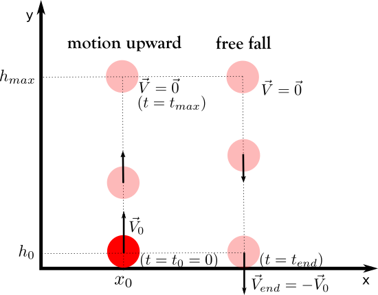
Below picture (fig 1) presents both types of motion:

Fig 1.

• Ad a. Ball is moving upward and then does free fall, when its initial velocity:

$\vec{V}_0=[0,V_y]$, where $V_y\gt 0$.

We can define key parameters that describe ball movement:

$t_0$ - time when movement starts (here $t_0=0$),
$t_{max}$ - time, when ball reaches highest height above the Earth's surface,
$t_{end}$ - time, when ball falls to the ground (moment of contact with Earth's surface),
$E_k$ - kinetic energy of ball,
$E_p$ - potential energy of ball,
$V_0$ - initial speed of ball ($V_0=|\vec{V_0}|$),
$V_{end}$ - speed of ball, when it contacts the ground,
$h$ - height of ball above the ground,
$h_0$ - initial height of ball laying on the ground. It equals to its radius $r$. If $r\ll h_{max}$, then $h_0\approx0$,
$h_{max}$ - max height of ball above the ground,
$g$ - acceleration of gravity (9.8 $m/s^2$). In our simulation we omit force due to air resistance. We can use energy conservation law, where only factors are potential and kinetic energy. Therefore: $$ E_p(t_{max})=E_k(t_0)=E_k(t_{end}) $$ $$ mgh_{max}=\frac{mV^2_0}{2}=\frac{mV^2_{end}}{2} $$ $$ h_{max}=\frac{V^2_0}{2g}=\frac{V^2_{end}}{2g} \tag{1}$$ We can come to conclusion: $$ V_0=V_{end}\tag{2}$$ Let's calculate $t_{max}$, $t_{end}$ now. To do this, we need to use formula for $h$: $$h=h_0+V_0t-\frac{gt^2}{2} \tag{3}$$ $t_{max}$ corresponds to $h_{max}$, therefore: $$h_{max}=h_0+V_0t_{max}-\frac{gt_{max}^2}{2} \tag{4}$$ Now, equation (1) needs to be put into formula (4). Finally $t_{max}$ is: $$t_{max}=\frac{V_0}{g} \tag{5}$$ Condition for $t_{end}$ looks like this: $$h_0=h_0+V_0\cdot t_{end}-\frac{gt_{end}^2}{2}$$ Therfore after simple calculations, $t_{end}$ is: $$t_{end}=\frac{2V_0}{g} \tag{6}$$ After comparison of $t_{max}$ with $t_{end}$, we can conclude that motion of ball, when it is first moving upward and then falls to the ground is completely symmetrical.


• Ad b. Ball does only free fall, when its initial velocity is $\vec{0}$ and initial position is above the ground.
Parameters that describe the ball's motion are:
$t_0$ - time when free fall motion starts,
$t_{end}$ - time, when ball falls to the ground (moment of contact with Earth's surface),
$V_{end}$ - speed of ball, when it contacts the ground,
$h$ - height of ball above the ground,
$h_0$ - initial height of ball above the ground.
Height $h$ is given by the formula: $$h=h_0-\frac{gt^2}{2} \tag{7}$$ We need to find parameters: $t_{end}$ and $V_{end}$. Condition for $t_{end}$ is: $$0=h_0-\frac{gt_{end}^2}{2}$$ Finally, $t_{end}$ is: $$t_{end}=\sqrt{\frac{2h_0}{g}} \tag{8}$$ Condition for $V_{end}$ is: $$mgh_0=\frac{mV_{end}^2}{2}$$ Finally, $V_{end}$ is: $$V_{end}=\sqrt{2gh_0} \tag{9}$$

Ad 2. Horizontal projection

Below picture (fig 2) presents this type of motion:

Fig 2.

Ball is moving in gravitational field according to horizontal projection motion, when its:

• initial position is above the ground level,
• has initial horizontal velocity $V_0$.

Ball's velocity is sum of vectors: $$\vec{V}=\vec{V}_0+\vec{V}_g, \tag{10}$$ where:
$\vec{V}_0=[V_0,0]$ - initial horizontal velocity, $\vec{V}_g=-gt$ - velocity caused by gravitational acceleration.

Parameters, that describe horizontal projection:
$t_0$ - time when horizontal projection starts,
$t_{end}$ - time, when ball falls to the ground (moment of contact with Earth's surface),
$V$ - ball's speed,
$V_{end}$ - speed of ball, when it contacts the ground,
$h$ - height of ball above the ground,
$h_0$ - initial height of ball above the ground,
$d$ - distance that ball moves.

Height $h$ is given by the same formula as free fall (equation (7)).
We need to find parameters: $t_{end}$, $V$, $V_{end}$, $d$.
$t_{end}$ is actually identical with $t_{end}$ for free fall motion (given by equation (8)) Based on formula (10), we can calculate speed of ball $V$: $$V=|\vec{V}|=\sqrt{V_0^2+(gt)^2} \tag{11}$$ Condition for $V_{end}$ is energy conservation law: $$mgh_0+\frac{mv_0^2}{2}=\frac{mV_{end}^2}{2}$$ Finally, after calculations we get: $$V_{end}=\sqrt{V_0^2+2gh_0} \tag{12}$$ Distance $d$ that balls reaches is pretty easy to figure out. It is just $V_0t_{end}$: $$d=V_0\sqrt{\frac{2h_0}{g}}. \tag{13}$$.

Ad 3. Angular projection

Below Fig 3. presents this type of ball's motion:

Fig 3.

Parameters, that describe angular projection are:
$t_0$ - time when angular projection starts,
$t_{max}$ - time after which ball reaches $h_{max}$,
$t_{end}$ - time, when ball falls to the ground (moment of contact with ground level),
$V$ - ball's speed,
$\vec{V_0}$ - initial ball's velocity vector,
$V_0$ - initial speed of ball,
$\alpha$ - angle between initial velocity vector $\vec{V}_0$ and ground level,
$V_{end}$ - speed of ball, when it contacts the ground (in $t=t_{end}$ moment),
$h$ - height of ball above the ground,
$h_0$ - initial height of ball laying on the ground. It equals to its radius $r$. If $r\ll h_{max}$, then $h_0\approx0$,
$h_{max}$ - max height of ball above the ground,
$d$ - distance that ball moves.

Initial velocity vector $\vec{V}_0$ can be present in general form: $$\vec{V}_0=[V_{0x},V_{0y}].$$ We can present initial velocity vector's components by $\alpha$ angle and its length $V_0$ as follows: $$ \begin{cases} V_{0x}=V_{0}\cdot cos(\alpha)\\ V_{0y}=V_{0}\cdot sin(\alpha) \end{cases} \tag{14}$$ Therefore, height of ball $h$ is: $$h=\underbrace{V_{0}\cdot sin(\alpha)}_{V_{0y}}\cdot t -\frac{gt^2}{2} \tag{15}$$ To calculate $h_{max}$ we use as usual energy conversation law: $$mgh_{max}+\frac{m\overbrace{V_0^2cos^2(\alpha)}^{V_{0x}^2}}{2}=\frac{mV_0^2}{2}$$ After basic calculations, we get: $$h_{max}=\frac{\overbrace{V_0^2\cdot sin^2(\alpha)}^{V_{0y}^2}}{2g} \tag{16}$$ To calculate $V_{end}$ we use energy conversation law again: $$\frac{mV_0^2}{2}=\frac{mV_{end}^2}{2}.$$ Based on above equation, we can easily conclude that: $$V_{end}=V_0. \tag{17}$$ To calculate $t_{max}$ we use equation (15) to create proper condition: $$h_{max}=V_{0y}t_{max}-\frac{gt_{max}^2}{2}. $$ $h_{max}$ is known because we calculate it before. It can be put to above equation: $$\frac{V_{0y^2}}{2g}=V_{0y}t_{max}-\frac{gt_{max}^2}{2}. $$ Finally, after basic calculations, $t_{max}$ is: $$t_{max}=\frac{V_{0y}}{g}. \tag{18}$$ Based on equation (15), we can write condition for $t_{end}$ parameter: $$0=V_{0y}\cdot t_{end}-\frac{g\cdot t_{end}^2}{2}.$$ After simple transformations we get: $$t_{end}=\frac{2V_{0y}}{g}. \tag{19}$$ We can easily figure out that $t_{end}=2\cdot t_{max}$, which means that angular projection motion is completely symmetrical.
Distance of ball $d$ is given by similar equation to eq(13): $$d=V_{0x}\cdot t_{end}= V_0cos(\alpha) \cdot \frac{2V_{0y}}{g}.$$ After simple calculations we get final version: $$d=\frac{V_0^2}{g}sin(2\alpha). \tag{20}$$

Simulation #1: 2D Pool game (part 2 - program)

In this article, I am going to describe program, that realizes 2D pool simulation.

Language that I chose is Python. I like it, because writing process is fast: it has concised syntax and many built in helpful methods. I am aware that it doesn't belong to fastest languages, but I think that it is completely enough fast to realize this task.

Program consists of 3 classes: Ball, Table and Simulation. Simulation class realize GUI besides running simulation. Below, I described in the form of table, content of each class:

Class: Ball
Variables	Description
t	time
dt	time step
x0,y0	initial coordinates of the ball (t=0)
vx0,vy0	initial velocity of the ball (t=0)
x,y	current ball coordinates
vx,vy	current ball velocity
R	radius of the ball
id	ball number (id)
color	ball color, for example "blue"
collisionBallNr	id of ball that collids with current ball
ifCollisionCompleted	variable of Boolean type, returns True if collision with ball is completed
Methods	Description
nextStep	calculates next ball position after dt (according to equation (0) from part 1)
ifCollisionWithBall	check if collision with ball happened, if yes - it calculates new velocities for it
ifCollisionWithEdge	check if collision with edge of the table happened, if yes - it calculates new velocities for it
setInitialBallVelocity	set random initial velocity for the ball

Class: Table
Variables	Description
L, W	table dimentions
borderCoordinatesX	array contains 2 edge values of x variable - that are: 0 and L
borderCoordinatesY	array contains 2 edge values of y variable - that are: 0, W
N	number of balls
balls	array that contains Ball objects
colors	array contains name of colors
Methods	Description
setInitialBallsPositions	set initial random positions for all balls, in a way that they do not overlap themself
actualPosition	run next step of simulation, i.e. run methods: nextStep, ifCollisionWithEdge, ifCollisionWithBall, returns actual position after the step
actualVelocity	auxiliary method, returns actual velovity of selected ball
getInitialPositionsAndVelocities	auxiliary method, returns initial velocities of all balls

Class: Simulation
Variables	Description
t	time
ifSimulationWorks	auxiliary variable of boolean type
ifPause	auxiliary variable of boolean type
Methods	Description
getNDt	gets N and dt variables from input fields
runSimulation	runs simulation
stop	stops simulation

The program window and the working simulation are finally presented as follows:

You can find project source and executable file on github: https://github.com/sim-num/2DpoolGameSimulation

Steps to program simulation:

1. Set initial values for each ball (position and velocity)
2. Calculate new position according to equation (0) from part 1
3. Check if collision with another ball or with the edge of the table occures (if yes - calculate new velocity)
4. Go back to step 2.

• Ad 1. Velocity initialisation (in class Ball):

  
      def setInitialBallVelocity(self):
          self.vx0 = random.randint(-10, 10)
          self.vy0 = random.randint(-10, 10)
          self.vx = self.vx0
          self.vy = self.vy0
         
   

  Initial velocity vector components are initialised with random integer values from range (-10, 10). Initialisation of position vector is realised by following method (in class Table):

  
      def setInitialBallsPositions(self, balls):
  
          for i in balls:
              while i.x0 == -1 and i.y0 == -1:
                  x = random.randint(i.R, Table.L - i.R)
                  y = random.randint(i.R, Table.W - i.R)
                  for j in balls:
                      if i.id != j.id and x <= (j.x + 2 * j.R) and y <= (j.y + 2 * j.R) and x >= (
                              j.x - 2 * j.R) and y >= (j.y - 2 * j.R):
                          x = -1
                          y = -1
                  i.x0 = x
                  i.y0 = y
                  i.x = i.x0
                  i.y = i.y0
         
   

  To initialise ball position, it is need to know other balls positions to avoid overlapping. This is the reason why position is initialised in class Table instead of Ball. We search for not overlapped position until it is found (while loop is used for that reason).
• Ad 2. Calculation of new position is performed by following method (in class Ball):

    def nextStep(self):
        self.x = self.x + self.vx * Ball.dt
        self.y = self.y + self.vy * Ball.dt
       
 

As you can easily see, equation (0) is programmed inside method nextStep. Second method that calculate next position is method called actualPosition inside class Table. It just calls method nextStep as well as other methods related to collision handling (see point 3).

    def actualPosition(self, ballNr, t):

        for i in range(0, self.N):
            self.balls[i].nextStep()
            self.balls[i].ifCollisionWithEdge()
            self.balls[i].ifCollisionWithBall(self.balls)
        return [self.balls[ballNr].x, self.balls[ballNr].y]
       
 

After ball move due to calling nextStep method, ifCollisionWithEdge and ifCollisionWithBall methods modify velocity vector appropriately if the collision conditions are met.
• Ad 3. Methods ifCollisionWithEdge and ifCollisionWithBall as said before are responsible for collision handling. Both belongs to class Ball. First method ifCollisionWithEdge is responsible for collision handling with edge. According to theory (see case 1 in part 1), depending on whether ball collids with vertical or horizontal edge of the table - respectively $V_x$ or $V_y$ component changes:

    def ifCollisionWithEdge(self):
        if self.x + self.R >= Table.borderCoordinatesX[1] and self.vx > 0:
            self.vx = -self.vx
        if self.x - self.R <= Table.borderCoordinatesX[0] and self.vx < 0:
            self.vx = -self.vx
        if self.y - self.R <= Table.borderCoordinatesY[0] and self.vy < 0:
            self.vy = -self.vy
        if self.y + self.R >= Table.borderCoordinatesY[1] and self.vy > 0:
            self.vy = -self.vy
       
 

ifCollisionWithBall is most complex method in program. Bellow is description step by step, how is it programmed (flag variable called ifCollisionCompleted is initialised in __init__ class method with value False):
1. Calculate distance between ball and another ball (for loop over all balls)
2. If distance is smaller than 2R and ifCollisionCompleted is False, then go to 3. else set ifCollisionCompleted to False for both balls and go back to step 1
3. Calculate $\alpha$ angle. It is related to arctan function as shown in part 1.
4. Calculate normal and tangent component of velocity vector for both collided balls (use equation (1b) from part 1.)
5. Swap normal component of velocity vector between balls.
6. Set ifCollisionCompleted flag to True for both balls.

    def ifCollisionWithBall(self, balls):  
        Xcoll = 0
        Ycoll = 0
        distanceFromBall = 99999
        for i in balls:
            if i.id != self.id:
                distanceFromBall = sqrt((self.x - i.x) ** 2 + (self.y - i.y) ** 2)
                if distanceFromBall <= 2 * self.R and self.ifCollisionCompleted == False:
                    self.collisionBallNr = i.id
                    Xcoll = (self.x + i.x) / 2
                    Ycoll = (self.y + i.y) / 2
                    alpha = 3.14159 / 2 - atan(float(self.y - i.y) / (self.x - i.x))  # collision angle

                    Vs = cos(alpha) * self.vx - sin(alpha) * self.vy
                    Vn = sin(alpha) * self.vx + cos(alpha) * self.vy
                    Vs_i = cos(alpha) * i.vx - sin(alpha) * i.vy
                    Vn_i = sin(alpha) * i.vx + cos(alpha) * i.vy
                    Vn_po = Vn_i
                    Vni_po = Vn
                    self.vx = cos(alpha) * Vs + Vn_po * sin(alpha)
                    self.vy = cos(alpha) * Vn_po - sin(alpha) * Vs
                    i.vx = cos(alpha) * Vs_i + Vni_po * sin(alpha)
                    i.vy = cos(alpha) * Vni_po - sin(alpha) * Vs_i
                    i.ifCollisionCompleted = True
                    self.ifCollisionCompleted = True
                elif distanceFromBall > 2 * self.R and self.ifCollisionCompleted == True and i.id == self.collisionBallNr:
                    self.ifCollisionCompleted = False
                    i.ifCollisionCompleted = False
       
 

Please notice that flag ifCollisionCompleted is static variable, which means that it is sufficient to set it by any of 2 collided balls. It should be like that, because if first ball ends the collision - second should know it.

Simulation visualisation

To visulize simulation I used Tkinter python library. Visualisation is implemented in method runSimulation, which belongs to class Simulation.

    def runSimulation(self):
        self.getNDt()
        self.ifPause = False
        if self.ifSimulationWorks == False:
            self.ifSimulationWorks = True
            while self.ifSimulationWorks:
                position = []
                velocity = []
                N = self.N
                for i in range(0, N):
                    position.append(self.Table.actualPosition(i, self.t))
                    velocity.append(self.Table.actualVelocity(i, self.t))
                ballSymbol = []
                velocityWektor = []
                for i in range(0, N):
                    ballSymbol.append(canvas.create_circle(position[i][0], position[i][1], 25, width=2,
                                                           fill=self.Table.balls[i].color, tags=('ball' + str(i))))
                canvas.update()
                canvas.after(40)
                for i in range(0, N):
                    canvas.delete(ballSymbol[i])

                self.t += 1
       
 

position and velocity arrays are used to keep position and velocity vector for all balls and t moment of simulation. Based on those values we can draw balls on screen on those positions and draw velocity vectors (however it is not implemented now). To draw balls we can use modified create_oval function:

def _create_circle(self, x, y, r, **kwargs):
    return self.create_oval(x - r, y - r, x + r, y + r, **kwargs)

tk.Canvas.create_circle = _create_circle
       
 

Modified function allows you to draw circles in the indicated position, which is the center of circle as well. Created ball symbol is stored in ballSymbol array. canvas.after(40) line causes sleep of 40 ms. It means that each t moment will last 40 ms. This value can be changed of course. If value is smaller then simulation will be more smooth, but slower because more calculations will be performing. Next, section:

                for i in range(0, N):
                    canvas.delete(ballSymbol[i])       
 

deletes all balls for t moment to make place for balls from t+1 moment.

Summary

Simulation is done according to my own idea. I hope it can be improved, code can be more concised. Maybe flag variables are not needed in this case. I am fan of simple code. I am really open to see other ways. Please leave comment if you have any suggestions.

Simulation #1: 2D Pool game (part 1 - theory)

At the beginning, I would like to deal with pool game simulation in 2 dimensions.

Simulation is based on right implementation of system of balls moving in area of rectangle that symbolizes table. What is most essential and hardest to do for this simulation is to calculate velocity vector $\vec{V}$ for each ball in each moment. When it is done, it is easy to calculate position vector $\vec{r}$
Rectangle that symbolizes table has dimentions $LxW$. In its area, there are $N$ balls with radius $R$. Balls should bounce with each other and from table borders. We assume that, all colissions are elastic. Therefore in this case, considering the fact also that system is close the total momentum is constant. We can apply law of Conservation of Energy here as well, where energy of the system is only kinetic energy of the balls. We assume that balls have the same mass. Other parameters for this simulation:

$\vec{r}_0=[x_0, y_0]$, $\vec{V}_0=[V_{x0}, V_{y0}]$ - respectively initial position and velocity of ball
$\vec{r}(t)=[x(t), y(t)]$, $\vec{V}(t)=[V_{x}(t), V_{y}(t)]$ - respectively actual position and velocity of ball

Let's define time step $\delta t$. Ball position at the moment of t $\vec{r}(t)$ is: $$\vec{r}(t)=\vec{r}(t-\delta t)+\vec{V}(t-\delta t)\cdot\delta t \tag{0}$$ We can easily see, that position at moment of $t$ depends on position in the previous time step, i.e. $t-\delta t$ and on velocity vector. Velocity vector depends on time as well. Because we omit friction, a single ball, if it does not encounter an obstacle, moves in a straight linear motion, i.e. its velocity vector is constant. Vector $\vec{V}$ changes when it encounters an obstacle, that is:

1. ball collids with the edge
2. ball collids with another ball

Let's analyze case number 1 - collision with edge:

Velocity vector of ball before collision we can present as pair of components: $V_x$ and $V_y$. Next, we can treat 2D case as two separate 1D cases along $x$ and $y$ axis respectively. Because motion along $y$ axis has direction parallel to the edge (when consider collision on left or right edge), so $V_y$ component remains the same after collision: $V_y'$=$V_y$. In case of $x$ axis, we have collision with the edge in this direction. It is an analog to collision with another ball with infinite big mass. According to fact that total momentum is constant, therefore velocity after collision in this direction is $V_x'$=$-V_x$, so it this the same as before collision but with minus sign. After collision with top or bottom edge we have opposite situation. Component $V_y$ is changed to $-V_y$ and $V_x$ remains same.

Case 2 - collision with another ball:
This case is more complex, because it requires entering the reflection angle to calculation. It depends on it, how velocity components of both balls are added. Only the components of the velocity vector change in the normal direction (denoted $V_n$) to the point of contact of the balls $P_s$ during the collision. Components in the tangent direction $V_s$ remain unchanged. This is shown in the figure below:

Fig.2

Knowing the values of normal components, the reflection boils down to one-dimensional reflection. We set initial velocities for balls (let's call them 1 and 2) as input parameters for the simulation, respectively: $\vec{V_1}=[V_{x1},V_{y1}]$ oraz $\vec{V_2}=[V_{x2},V_{y2}]$. In order to calculate normal and tangent components, we need to express these vectors in the new coordinate system denoted by Fig. 2 through $x'$, $y'$. We can see in the figure that it is rotated in trelation to the $x$, $y$ system by the angle $\alpha$
To transform from one system to another, we use general formula for coordinate transform: $$\begin{cases}x'=xcos(\alpha)-ysin(\alpha)\\ y'=xsin(\alpha)+ycos(\alpha)\end{cases} \tag{1}$$ The angle $\alpha$ can easily be calculated, knowing that $tg(90^{\circ}-\alpha)=ctg(\alpha)$ is the The angle $\alpha$ can easily be calculated to know that $ tg(90^{\circ} - \alpha) = ctg (\alpha) $ is the slope of the line passing through the centers of balls and whose coordinates we know because they mark the position of our balls on the table. Finally, $\alpha=acrctg(\frac{y_1-y_0}{x_1-x_0})$. General formula for normal and tangent component of velocity vector for the first ball is thus: $$\begin{cases} V_{1s}=V_{1x}cos(\alpha)-V_{1y}sin(\alpha) \\ V_{1n}=V_{1x}sin(\alpha)+V_{1y}cos(\alpha)\end{cases} \tag{1b}$$ Analogously for the sphere no. 2. As I mention above, after the collision tangent component remain unchanged. Normal components swap, i.e. $V_{1n}'$ denotes normal component of velocity vector for ball no. 1 after collision is equal to normal component for ball no. 2 before collision: $ V_ {1n}' = V_ {2n} $. Similarly $V_{2n}'$ for ball number 2. Finally, normal and tangent component for both balls after collision: $$ \begin{cases} V_{1s}'=V_{1x}cos(\alpha)-V_{1y}sin(\alpha) \\ V_{1n}'=V_{2x}sin(\alpha)+V_{2y}cos(\alpha)\\ V_{2s}'=V_{2x}cos(\alpha)-V_{2y}sin(\alpha)\\ V_{2n}'=V_{1x}sin(\alpha)+V_{1y}cos(\alpha) \end{cases}\tag{2}$$ Finally, it remains to go back to the original coordinate system to present the velocity vector components of the two balls after reflection. For this purpose, we will again use the formulas (1). Ultimately, the components of the velocity of the balls after reflection reflect the following formula: Finally, we need to get back to initial dimentional system to present the velocity vector components of the two balls after collision. For this purpose, we will use the formulas (1) again. Ultimately, velocity components of the two balls after collisions are determined by the folowing formulas: $$ \begin{cases} V_{1x}'=V_{1s}'cos(\alpha)+V_{1n}'sin(\alpha) \\ V_{1y}'=V_{1n}'cos(\alpha)-V_{1s}'sin(\alpha) \\ V_{2x}'=V_{2s}'cos(\alpha)+V_{2n}'sin(\alpha) \\ V_{2y}'=V_{2n}'cos(\alpha)-V_{2s}'sin(\alpha) \end{cases} \tag{3}$$ It is enough now to put the formulas (2) into equations (3) to obtain the final form of the velocity components after mutual ball collision. This is as an aside, because we use a programming language, we can assign values to variables, so we do not need to know the final analytical form.